Exploring CO2 emissions from space
At industry facilities such as power plants and smelters, CO2 is mostly produced by combustion of fossil fuels such as coal, peat, petroleum, and natural gas. Power plants and smelters combust these fossil fuels to produce electricity for our homes or to create heat in furnaces for metal extraction, respectively.
Tracking the CO2 activity at such industry facilities is important for 3 major reasons:
It enables analysis and comparison between the anthropogenic production of greenhouse gas emissions and pollution of our atmosphere.
It provides companies that manage or invest in these operations insight into what activity is going on at each of their locations of interest.
It provides a means for the individual facilities to monitor their own production activity and gas emissions, enabling more effective reporting on GHG emissions to meet regulatory constraints.
There are many methodologies that scientists can use in order to measure CO2 concentrations in our atmosphere, including ground-based, aerial, and satellite measurements.
At Sust Global, we chose to run an exploratory analysis of CO2 emissions in the atmosphere above power plants and smelters by using the OCO-3 instrument aboard the international space station. We decided on the OCO-3 instrument because it provides daily measurements of CO2 concentrations globally, with repeat analyses every 16 days. By using the OCO-3 dataset, we can therefore track atmospheric CO2 contents in a temporally frequent manner at global scale.
Most often, the OCO-3 dataset and its predecessor, the OCO-2 dataset, are used to construct global maps such as the map shown below. Such global maps can be useful for showing global and seasonal trends of CO2 within the atmosphere.
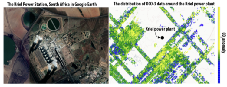
Image of the Kriel Power Station in South Africa that we used as a case study. The OCO-3 data occurs in narrow swaths and does not cover large portions of Earth. The Kriel power plant is shown to be within an area that is not directly covered by OCO-3 data.
We decided to use the geospatial interpolation method called kriging to deal with areas of missing data. Kriging was previously explored and proved effective for L3 XCO2 estimation. (Cressie, 2016). To understand how this works, imagine the data set of atmospheric CO2 concentrations is a large data grid. In some cases, the grid contains CO2 concentrations measured with OCO-3, and in some cases there are no values available.
Kriging can be used to interpolate the statistically best predictions of values in the empty grid cells by using the data in the filled grid cells. In this way, kriging can fill out each part of the grid and calculate the variance, a measurement of uncertainty, for each calculated grid value.
Below you can see how the kriging method was used to calculate values for all of the places where OCO-3 had not made any measurements. Note that when data is very sparse, the uncertainty in the form of variance is high, as expected.
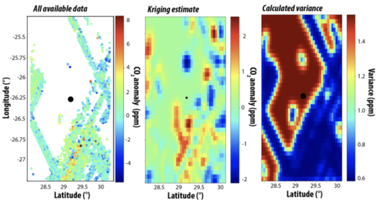
Results after performing kriging interpolations for the area surrounding the Kriel power plant. The original data available from OCO-3 can be seen in the middle panel, while the fully interpolated grid after kriging is shown in the left panel. The variance of the kriging estimates are shown to the right.
Kriging methods are performed by using a gaussian process governed by a covariance model that is often represented by a variogram. A variogram shows the variance between two different spatial locations of interest. The distance between the two locations is often referred to as the lag distance. This is an example of one of the variogram models that were used for our kriging method.
Constructing a reliable model for the variogram can be quite a challenge, as the CO2 anomaly is often very varied from data point to data point. This can cause quite a lot of variability in the closely spaced data, from which the kriging algorithm is trying to interpolate.
As we looked at regions that were quite small with a lot of data sparsity and closely-spaced data variability, this became a very difficult task. The kriging algorithm worked in some cases, like the instance shown, but may not be reliable from location to location.
When there’s large gaps in data, the kriging algorithm may just interpolate a mean value for large swaths, observed in the results above, that could, in theory, be substituted with the calculation of a simple mean.
From the results of the kriging algorithm, we calculated the quarterly mean and standard deviation for the Kriel power plant and a reference location. An uninhabited area was picked as the reference location so it would be less likely to be influenced by anthropogenic emissions, with ~1 deg (or 111 km) from the Kriel power plant.
Analysis can only really be performed on a QoQ or YoY basis. The data from OCO-3 is simply too sparse to be useful on a monthly basis, which cannot yield reliable interpolation with kriging.
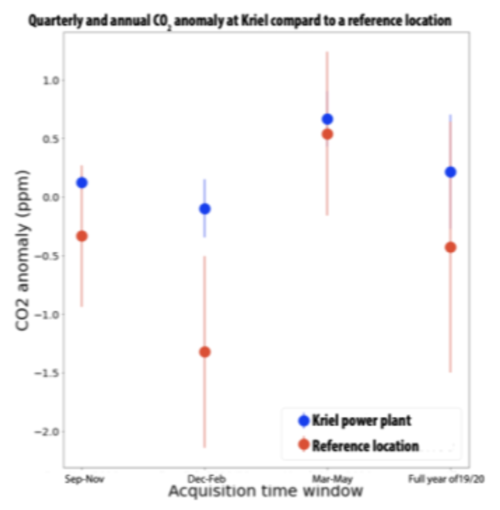
Krigged estimates of the quarterly CO2 anomalies in the atmosphere surrounding the Kriel power plant compared to an uninhabited reference location. Note that the uncertainty of the krigged estimate is quite high, but that the CO2 anomaly is generally higher around the Kriel power station compared to an uninhabited reference location, as expected.
Issues that we encountered using our kriging algorithm, led us to investigate the Total Carbon Column Observing Network (TCCON) data set. The TCCON data set is a ground-based network of 25 spectrometers that measure greenhouse gasses, including CO2.
These measurements are more precise than satellite-based measurements but do not offer a lot of spatial coverage. They can be used as calibration points for satellite datasets. We checked the TCCON measurements against our OCO-3 measurements and found that both seasonal trends and CO2 anomalies matched well with each other. This suggested that L2 OCO-3 data was good at replicating the ground-based measurements.
However, we did see that there was a large variability associated with the daily CO2 anomaly when performing averaging and standard deviation calculations of both the TCCON and OCO-3 data sets. Because the concentration of CO2 was generally high in the atmosphere, we found that small changes in daily CO2 concentrations by individual industry facilities can be very difficult to track.
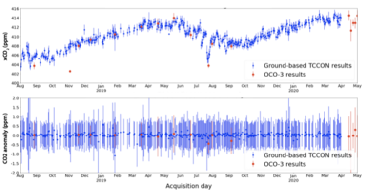
Daily averages and standard deviation of measurements from the Lamont TCCON station in Oklahoma in blue compared to measurements extracted from OCO-3 and OCO-2 datasets in red. The upper panel shows measurements with no background removal revealing a seasonal signal. The lower panel shows the background removed values producing the CO2 anomaly.
As explored in the plot above, we also incorporated the datasets from the OCO-2 mission into our analysis. The OCO-2 dataset is largely similar to the OCO-3 but was created by a satellite rather than by an instrument aboard the international space stations.
Therefore, the flight paths and swath sizes are often observed to be different to the OCO-3 data, although the data structure is largely similar. Importantly, the OCO-2 mission has been operating since 2014, whereas the OCO-3 mission has only been operating since 2019. Using the OCO-2 data gave us access to more historical data. The tradeoff being that more data meant the process would be more computationally intensive.
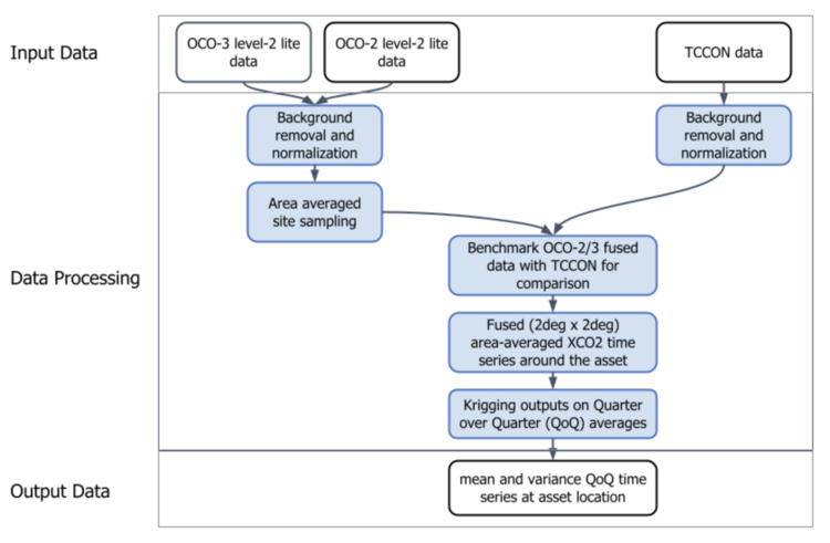
Proposed data processing pipeline integrating OCO-2, OCO-3, and TCCON data sets, performs and kriging, and allows QoQ and YoY time series analysis.
By integrating the OCO-2, OCO-3, and TCCON data as well as kriging methodologies, we created a workflow that uses state-of-the-art datasets to explore future changes to anthropogenic emissions within the atmosphere, no matter how small. The resulting asset-level CO2 estimates are integrated into our product offerings.
To reiterate, the primary data challenges we encountered with the proposed workflow are:
1. OCO-3/OCO-2 data were primarily designed for global maps. Therefore, typical single asset locations are too small to be reliably detected in the OCO-2/OCO-3 data with large temporal and spatial data gaps.
2. The high local variability in OCO-2/OCO-3 data and large data gaps complicate kriging performance.
3. Anthropogenic emissions of CO2 is a relatively weak signal compared to natural background CO2 concentrations due to the long residence time of CO2, resulting in little variability and high comparative uncertainties when working in background-removed CO2 anomaly space.
Here are some opportunities to further improvements to the data analysis pipeline:
1. Geospatial data fusion with alternate data sources that estimate CO2 emissions, like ground-based stations.
2. Improved spatial record of OCO-3 data by longer collection time.
3. Choosing larger CO2 hotspots as regions of interest such as cities, harbors and clusters of power plants for further calibration.
Sust Global transforms complex climate science into meaningful financial indicators. To learn more about how we can help you with your sustainability goals, get in touch by completing the form below.